Diagnostic Validity – by Andrew Cuff

Our articles are not designed to replace medical advice. If you have an injury we recommend seeing a qualified health professional. To book an appointment with Tom Goom (AKA ‘The Running Physio’) visit our clinic page. We offer both in-person assessments and online consultations.

A big part of physiotherapy is understanding evidence-based practice. It can be a confusing and complex area. Luckily physios like Andrew Cuff are producing some great work to help us make sense of it. Andrew has created Applying Criticality – an excellent site designed to help physios develop their critical appraisal skills. So I was delighted when he kindly agreed to produce a guest blog for us on the reliability and validity of diagnostic tests. This is part of the site’s Physio Resources – designed to help share knowledge and research between clinicians (as Andrew says below it’s one for the physios rather than the runners!)

Andrew is an experienced Physio, 2:45 marathon runner and research commentator with @evbasedphysio. You can follow him on Twitter via @AndrewVCuff and I highly recommend his previous work; Research Questions and Clinical Reasoning, What is Evidence-Based Practice? and Searching the Literature

Once again we’ve teamed up with @PDPhysios and @PDPhysios2 to share this page with others to help with CPD;

Tom invited me to guest blog on this subject at the perfect time – I’d just finished an MSc module looking at measurement in clinical practice so the theory and the application are relatively fresh! I must thank Joe Palmer, former First Team Physiotherapist at Sheffield United for sharing some material with me and acknowledge that I was very fortunate to be taught by Dr Stephen May, a well-published researcher in the psychometric properties of physical examination components in both the Lumbar Spine and the Shoulder.

Validity and Reliability are concepts briefly touched upon during undergraduate Physiotherapy training and are concepts that a lot of Physiotherapists don’t have a great understanding of. I, therefore, aim to introduce the concepts and key terms in relation to diagnostic tests to develop a practical, clinical understanding in order to enhance clinical application. If you are an athlete reading this, you may want to skip this post – I’ve just added a whole new boring dimension to RunningPhysio!

What is Reliability?

Reliability refers to the measure of the consistency of the results obtained when a measure is used at two separate points in time or by two different individuals; Without reliability, we cannot make a definitive conclusion about the results that we obtain.

Inter-rater reliability– Agreement on a result between two or more assessors

Intra-rater reliability– Agreement between results obtained by the same assessor at two separate time points.

Inter-rater reliability is deemed to be more important as this takes into account all potential errors encountered within intra-rater reliability as well as the potential for error between clinicians. Therefore, high inter-rater reliability would be suggestive of high intra-rater reliability (High intra-rater reliability, however, does not suggest high inter-rater reliability!).

How is Reliability Measured and Interpreted?

This relates to the percentage of agreement observed between raters and excludes the likelihood of the agreement occurring due to chance. This is calculated using a reliability coefficient.

These vary depending on the type of data produced by the measurement tool however, with this article focusing on the reliability of physical examination diagnostic/special tests I won’t bore you with these obscure details!

A ‘reliability coefficient’ is used to measure reliability and in turn aid interpretation: For diagnostic tests consisting of a positive or negative finding (i.e. nominal data) a Kappa Coefficient is used for both inter and intra-rater reliability.

All reliability coefficients are interpreted in the same way:

• 1.0 (100%)- All raters achieve exactly the same result (perfect agreement).
• 0 (0%)- The results obtained from different raters are no better than those predicted by chance (no agreement).
• Negative results- The results agreed on between different raters are less than those predicted by chance.
• 0.75 is generally the minimal acceptable figure for reliability (Streiner and Norman, 2003)

It is important to ensure that when testing reliability, and when reading articles that are testing reliability, that all assessors must be blinded from each other’s results. A lack of independence on the part of the assessors may alter the true representation of results, impacting on the final Kappa value, either positively or negatively (i.e. increasing the result towards 1.0 or lowering it).

How much reliability is enough?

• 0.0 – 0.2 = poor
• 0.2 – 0.4 = fair
• 0.4 – 0.6 = moderate
• 0.6 – 0.8 = good
  
• 0.8 – 1.0 = very good

(Landis and Koch 1977)

Validity

Validity can be discussed in the context of either a piece of research or a particular type of measure; in order to minimise confusion, both are outlined below.

Research Validity

The validity of a study (e.g. an RCT) can be divided into two categories

• Internal validity– A measure of how well the results of a study can be trusted.
• External validity– Are the result generalizable to a wider population?

Measurement Validity

Refers to how well something measures what it is intended to measure. In the context of diagnostic testing, it is the ability of the test to achieve a correct diagnosis. It is therefore specific to a particular patient group or condition. With this is mind, the important question should not be ‘Is this measure valid?‘, but more ‘HOW VALID is this measure?‘

Although there are a number of components to validity, two are extremely relevant to diagnostic testing:

• Criterion Validity– How does the measure compare to the ‘Gold Standard‘ for diagnosis?
• Predictive Validity– Does the measure provide an accurate earlier prognosis than current instruments?

Criterion Validity

This is the most common form of validity that is encountered and is assessed quantitatively. It is used to compare an examination procedure to the ‘Gold Standard’; for example, assessing the criterion validity of the Lachmann’s test to Arthroscopic findings in diagnosing ACL rupture.

Criterion validity can be further subdivided into a number of categories; firstly:

Sensitivity– The ability of a diagnostic test to detect pathology WHEN THERE IS PATHOLOGY PRESENT.

Essentially meaning ‘Is the test sensitive enough to detect something?’ i.e. a True Positive.

A useful pneumonic that Dr May recommended using was ‘SnNout’, and is very useful to remember and keep in mind when reading reliability papers.

SnNout– A measure with High Sensitivity that finds a Negative result rules out an individual having pathology

Specificity– The ability of a diagnostic test to produce a negative finding in the ABSENCE OF PATHOLOGY

Essentially meaning ‘Is the test specific enough to a particular pathology that is able to detect those that do not have it?’ i.e. a True Negative

Another of Dr May’s pneumonics: SpPin

SpPin– A measure with High Specificity that finds a Positive result rules in an individual having pathology.

Measuring Sensitivity and Specificity

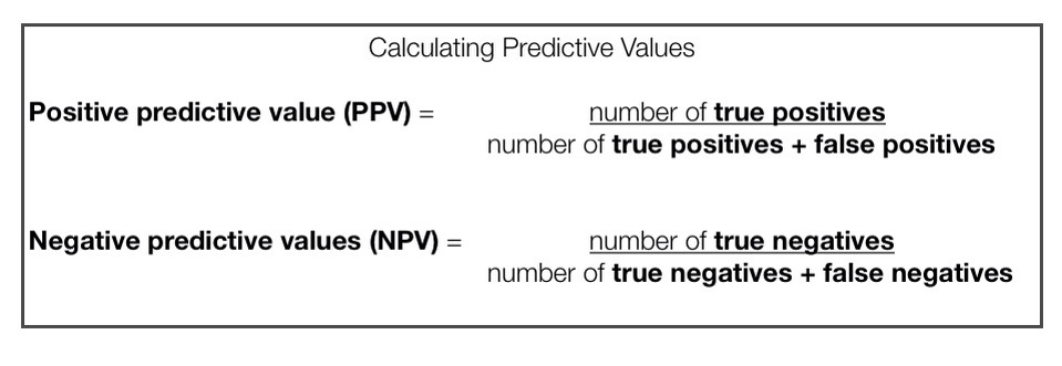
Results obtained from studies investigating the criterion validity of a diagnostic test can be displayed in a table that compares the findings of the technique to the ‘Gold Standard‘. The table below shows how findings would be presented.

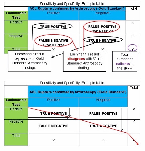
The black arrows show where the Lachmanns test has achieved the same findings as Arthroscopy and has therefore achieved a correct diagnosis.

EXAMPLE

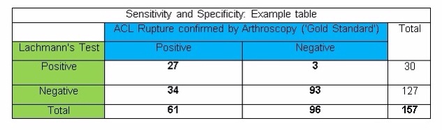
To demonstrate this visually and make sense of theory, the following example uses a comparison between the findings on a Lachmann’s test and the ‘Gold Standard’, definitive findings seen with Arthroscopy in diagnosing ACL rupture in a group of 344 patients.

The table below shows a FICTIONAL example. The data in the table IS NOT ACTUALLY RELATED TO THE LACHMANN’S TEST OR ACL INJURIES!!! From this point on the figures used in subsequent examples will relate to this table.

A perfect test would have a sensitivity and specificity of 100% or a kappa value of 1.0. HOWEVER, there tends to be a see-saw relationship between the two. – as one increases, the other tends to decrease as a result.

In conclusion

• Sensitivity and specificity tell us HOW GOOD a diagnostic test is.
• It is a measure of how likely a particular diagnosis is correct.
• Sensitivity and specificity DO NOT take into account the prevalence of a particular disease.

Aspects of Criterion Validity- Predictive Values

When we acknowledge the prevalence of a particular condition in conjunction with the criterion validity of a diagnostic test we end up with its PREDICTIVE VALUE. These are regarded as being more relevant clinically than criterion validity.

Predictive values can be subdivided into two groups:

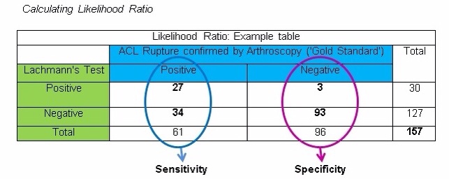
Positive Predictive Value (PPV): Proportion of patients who TEST POSITIVE and HAVE THE PATHOLOGY. The ability to detect a true positive.

Negative Predictive Value (NPV): Proportion of patients who TEST NEGATIVE and DO NOT HAVE THE PATHOLOGY. The ability to detect a true negative.

Aspects of Criterion Validity- Overall Accuracy

This simply related to the NUMBER OF CORRECT RESULTS the measure produces when compared to the ‘Gold Standard‘. It should be noted however that this is rarely used in practice as it is highly susceptible to change in the prevalence of pathology and sampling characteristics.

If we were to use the example table presented above to demonstrate this, it would look as follows:

‘Overall Accuracy’ = 27 + 93 = 120 … 120 / 157 = 0.764

‘Overall Accuracy’ = 76%

Aspects of Criterion Validity- Likelihood Ratio

The likelihood ratio provides information relating to the level of doubt from a given diagnosis. This is done by calculating the probability of ANY individual actually HAVING THE PATHOLOGY, despite the results of a diagnostic test. This can be subdivided into two categories:

• Positive Likelihood Ratio (PLR) – What is the probability of a patient who tests POSITIVE on a diagnostic test actually HAVING PATHOLOGY?
• Negative Likelihood Ratio (NLR) – What is the probability of a patient who tests NEGATIVE on a diagnostic test actually HAVING PATHOLOGY?

Step-By-Step

• Initially, the sensitivity and the specificity results of the test need to be converted into a percentage
  • E.g. 27 / 61 = 0.44 0.44 x 100 = 44% Sensitivity of 0.44
  • E.g. 93 / 96 = 0.97 0.97 x 100 = 97% Specificity of 0.97
• Secondly, add the figures (0.44 and 0.97) into the formulas shown below to perform the appropriate calculation.

Positive likelihood Ratio (PLR): Sensitivity / (1 – Specificity)

0.44 / (1 – 0.97) = 14.67

Negative likelihood Ratio (NLR): (1 – Sensitivity) / Specificity

(1 – 0.44) / 0.97 = 0.58

Significant Values for Likelihood Ratios– Rule of thumb

It is generally accepted that:

A Positive likelihood Ratio (PLR) >10 can RULE IN a diagnosis

A Negative likelihood Ratio (NLR) < 0.1 can RULE OUT a diagnosis

The fictional clinical conclusion that can be drawn from the example would therefore be that a negative Lachmann’s Test cannot rule an ACL Rupture, but a positive Lachmann’s Test can rule in an ACL Rupture.

Pre and Post-test Odds

It is possible to use the obtained likelihood ratio to particularise/tailor the results to each individual patient. As the likelihood ratio is a form of odds ratio, we must therefore use pre and post-test odds.

Calculating pre and post-test odds

Pre-Test odds/ probability is a statement of the likelihood that a patient with a particular presentation has a specific diagnosis

Pre-test Odds = Sensitivity / Specificity 0.44 / 0.97 = 0.45 (45%)

Once a test result has come back for a particular patient, the post-test odds can then be calculated by multiplying the pretest odds by either the Positive or Negative Likelihood Ratio (i.e. the PLR for a result that returns positive and the NLR for when a result returns Negative).

Post-test Odds/ probability are a statement of the likelihood that a patient has a diagnosis after the results of a test.

Post-test Odds (Positive test result) = Pre-Test Odds x PLR

0.45 x 14.67 = 0.03

Post-test Odds (Negative test result) = Pre-Test Odds x NLR

0.45 x 0.58 = 0.26

Fagans Nomogram

This is a form of graph which isn’t commonly seen in many research papers, understanding, reflecting and applying the above will give you sufficient ability to understand the results of a reliability study. However, in case you have been ‘lucky’ to see one, or will be ‘fortunate’ to see one in the future, I’ve tried to explain it as practically as I can!

The Fagans Nomogram allows Pre-Test Probabilities to be converted into Post-Test Probabilities for a diagnostic test if there is a given Positive or Negative Likelihood Ratio.

Plotting a Fagans Nomogram

1. Convert Pre-test result (Sensitivity / Specificity) into either percentage or odds, depending on the type of Nomogram using the formulas below:
   • Percentage = Odds / (odds + 1)
   • Odds = Percentage / (Percentage + 1)
2. Locate the Pre-Test value on the ‘Pre-Test Probability (%)’ column. This will be that starting point for both positive and negative Post-Test probability plot lines.
3. Locate the points on the ‘Likelihood Ratio’ scale at the centre of the Nomogram for both the PLR and the NLR.
4. Draw a straight line starting from the ‘Pre-Test probability value’, through the respective PLR and NLR values on the ‘Likelihood Ratio’ Scale until the line crosses the ‘Post-Test probability (%)’ column on the opposite side of the Nomogram,.

References

LANDIS, J. and KOCK, G. (1977). The measurement of observer agreement for categorical data. Biometrics, 33, 159-174.

NORMAN, Gregory and STREINER, David (2003). PrettyDarnedQuick Statistics. 3rd ed, London, BC Decker.